Quickstart
This section serves as quick demo how to use the library. The presented example can be found in the tests/demos directory of the repository inside demo_not-a-knot.py.
Data preparation
First, we need to prepare the data. In this example, we assume 2-dimensional sample values on a regular grid. The grid must be equidistant in each dimension. However, the grid spacing may differ between dimensions.
import numpy as np
import cubicmultispline as spl
import matplotlib.pyplot as plt
from matplotlib import cm

"""
Preparing dummy data
"""

# shape of the data -> number of points in each dimension
shape = (11, 9)

# ranges of the data -> [min, max] for each dimension
ranges = [
    [0, 1],
    [0, 0.8],
    ]

# interval tuple for each dimension -> (min, max, number of points) for each dimension
interval = tuple((ranges[i][0], ranges[i][1], shape[i]) for i in range(len(shape)))

# boundary conditions for each dimension -> (first condition, second condition) for each dimension
bc = (
    ("not-a-knot", "not-a-knot"),
    ("not-a-knot", "not-a-knot"),
    )

# boundary conditions values for each dimension -> (first condition value, second condition value) for each dimension
# for "not-a-knot" and "periodic" boundary conditions, the values are not used
bc_value = (
    (0.0, 0.0),
    (0.0, 0.0),
    )

# generation of random dummy data
dummy_data = np.random.randn(*shape).ravel()
Important
It is important, that the sample data is always a 1-dimensional array of length np.prod(shape). You can convert any multidimensional array using ravel(). This makes sure that the values are sorted correctly regarding the dimensions (first dimension changes slowest, last dimension changes fastest).
Spline generation and inspection
Next, the spline surface can be created:
# generation of spline surface
spline_2d = spl.Spline(interval, dummy_data, bc, bc_value)
Note
The sample positions are not passed explicitly. Instead, the interval tuple carries all necessary information.
In order to compare the generated spline to the sample data, we can evaluate the spline at the sample positions. To this end, the sample positions are generated using np.meshgrid:
"""
Preparing plotting
"""

# Locations of dummy_data samples
x_sample = np.linspace(ranges[0][0], ranges[0][1], shape[0])
y_sample = np.linspace(ranges[1][0], ranges[1][1], shape[1])
x_sample, y_sample = np.meshgrid(x_sample, y_sample, indexing='ij')
The spline can be evaluated at any point in the domain using the eval_spline() method. To achieve a smooth surface, we evaluate the spline on a finer grid:
# Locations of spline evaluations for smooth surface
x_spline_eval = np.linspace(ranges[0][0], ranges[0][1], shape[0]*50)
y_spline_eval = np.linspace(ranges[1][0], ranges[1][1], shape[1]*50)
x_spline_eval, y_spline_eval = np.meshgrid(x_spline_eval, y_spline_eval, indexing='ij')
The eval_spline() method returns the spline values, the gradient and the Hessian for each point. In this example, we only need the spline values vals:
# Spline evaluation
coords = np.concatenate((
    x_spline_eval.reshape((-1,1)),
    y_spline_eval.reshape((-1,1))
    ), axis = 1)
vals, dvals, ddvals = spline_2d.eval_spline(coords)
vals = vals.reshape(x_spline_eval.shape)
The resulting spline values are reshaped to match the shape of the evaluation grid for plotting purposes. Finally, we can plot the spline surface and the sample data:
# Plot dummy data and spline surface
fig = plt.figure()
plt.subplots_adjust(hspace=0.5, wspace=0.4)
ax = fig.add_subplot(111, projection='3d')
ax.plot_surface(x_spline_eval, y_spline_eval, vals, antialiased = True, alpha = 0.8, cmap = cm.Blues)
ax.scatter(x_sample, y_sample, dummy_data.reshape(x_sample.shape), c = "red", marker = 'x')

ax.set_xlabel('x')
ax.set_ylabel('y')
ax.set_zlabel('data')
plt.show()
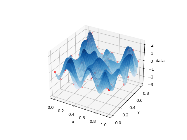
The resulting plot should look similar – not identical due to random data – to the following. The red crosses mark the random sample values.
More complex cases, which also discuss different boundary conditions, are found on the following pages.